No edit summary |
No edit summary |
||
| (20 intermediate revisions by 6 users not shown) | |||
| Line 4: | Line 4: | ||
[[Category:ODE]] | [[Category:ODE]] | ||
[[Category:time invariant]] | [[Category:time invariant]] | ||
[[Category: | [[Category:Parametric]] | ||
[[Category:affine parameter representation]] | [[Category:affine parameter representation]] | ||
[[Category:first differential order]] | [[Category:first differential order]] | ||
[[Category:SISO]] | |||
{{Infobox | |||
|Title = Anemometer | |||
|Benchmark ID = | |||
* anemometer1Param_n29008m1q1 | |||
* anemometer3Param_n29008m1q1 | |||
|Category = misc | |||
|System-Class = AP-LTI-FOS | |||
|nstates = 29008 | |||
|ninputs = 1 | |||
|noutputs = 1 | |||
|nparameters = | |||
* 2 | |||
* 5 | |||
|components = A, B, C, E | |||
|License = NA | |||
|Creator = [[User:Feng]] | |||
|Editor = | |||
* [[User:Feng]] | |||
* [[User:Himpe]] | |||
* [[User:Lnor]] | |||
* [[User:Baur]] | |||
* [[User:Will]] | |||
* [[User:Lund]] | |||
|Zenodo-link = NA | |||
}} | |||
==Description== | ==Description== | ||
<figure id="fig:plot1"> | |||
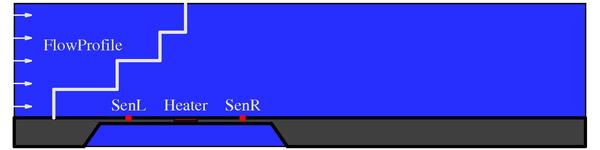
[[File:Model_Color.pdf|600px|thumb|right|<caption>Schematic 2D-Model-Anemometer</caption>]] | |||
</figure> | |||
<figure id="fig:plot2"> | |||
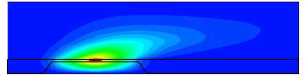
[[file:ContourPlot30.pdf|600px|thumb|right|<caption>Calculated temperature profile for the Anemometer function</caption>]] | |||
temperature | </figure> | ||
An '''Anemometer'''<ref name="ernst01" group="a)"/><ref name="benner05" group="a)"/><ref name="moosmann05" group="a)"/><ref name="moosmann07" group="c)"/><ref name="moosmann05b" group="c)"/><ref name="rudnyi06" group="c)"/> (see [[wikipedia:Thermal_mass_flow_meter|thermal mass flow meter]]) | |||
convection | is a flow sensing device, consisting of a heater and temperature sensors before and after the heater, placed either directly in the flow or in its vicinity Fig. 1. | ||
They are located on a membrane to minimize heat dissipation through the structure. | |||
Without any flow, the heat dissipates symmetrically into the fluid. | |||
This symmetry is disturbed if a flow is applied to the fluid, | |||
which leads to a convection on the temperature field and therefore to a difference between the temperature sensors (see Fig. 2) from which the fluid velocity can be determined. | |||
< | The physical model can be expressed by the [[wikipedia:Convection–diffusion_equation|convection-diffusion partial differential equation]] <ref name="moosmann04" group="b)"/>: | ||
:<math> | |||
\rho c \frac{\partial T}{\partial t} | |||
= \nabla \cdot (\kappa \nabla T) | |||
- \rho c v \nabla T | |||
+ \dot{q}, | |||
</math> | |||
where <math>\rho</math> denotes the mass density, <math>c</math> is the specific heat capacity, <math>\kappa</math> is the thermal conductivity, | |||
<math>v</math> is the fluid velocity, <math>T</math> is the temperature, and <math>\dot q</math> is the heat flow into the system caused by the heater. | |||
The solid model has been generated and meshed in [[wikipedia:ANSYS|ANSYS]]. | |||
Triangular [http://www.ansys.stuba.sk/html/elem_55/chapter4/ES4-55.htm PLANE55] elements have been used for the finite element discretization. | |||
The order of the system is <math>n = 29008</math>. | |||
Example with | Example with one parameter: | ||
The <math>n</math> dimensional ODE system has the following transfer function | The <math>n</math> dimensional [[wikipedia:Ordinary_Differential_Equation|ODE]] system has the following transfer function | ||
<math> | :<math> | ||
G(p) = C( | G(s, p) = C (s E - A_1 - p (A_2 - A_1))^{-1} B | ||
</math> | </math> | ||
with the fluid velocity <math>p(=v)</math> as single parameter. | with the fluid velocity <math>p(=v)</math> as single parameter. | ||
Here <math>E</math> is the heat capacitance matrix, <math>B</math> is the load vector which is derived from separating the spatial and temporal variables in <math>\dot{q}</math> and the FEM discretization w.r.t. the spatial variables. <math> | Here <math>E</math> is the heat capacitance matrix, <math>B</math> is the load vector which is derived from separating the spatial and temporal variables in <math>\dot{q}</math> and the [[wikipedia:Finite_Element_Method|FEM]] discretization w.r.t. the spatial variables. | ||
<math>A_i</math> are the stiffness matrices with <math>i=1</math> for pure diffusion and <math>i=2</math> for diffusion and convection. | |||
Thus, for obtaining pure convection you have to compute <math>A_2 - A_1</math>. | |||
Example with | Example with three parameters: | ||
Here, all fluid properties are identified as parameters. Thus, we consider the following transfer function | Here, all fluid properties are identified as parameters. Thus, we consider the following transfer function | ||
<math> | :<math> | ||
G(s, p_0, p_1, p_2) = | |||
C | |||
( | |||
s \underbrace{(E_s + p_0 E_f)}_{E(p_0)} | |||
- \underbrace{(A_{d,s} + p_1 A_{d,f} + p_2 A_c)}_{A(p_1,p_2)} | |||
)^{-1} | |||
B | |||
</math> | </math> | ||
with parameters <math>p_0, | with parameters <math>p_0</math>, <math>p_1</math>, <math>p_2</math> which are combinations of the original fluid parameters <math>\rho</math>, <math>c</math>, <math>\kappa</math>, <math>v</math>: <math>p_0 = \rho c</math>, <math>p_1 = \kappa</math>, and <math>p_2 = \rho c v</math>, see <ref name="baur11" group="c)"/>. So far, we have considered the mass density as fixed, i.e. <math>\rho=1</math>. | ||
==Origin== | ==Origin== | ||
IMTEK Freiburg, group | * [http://www.imtek.uni-freiburg.de/professuren/simulation/ IMTEK Freiburg, Simulation group], Prof Dr Jan G. Korvink has taken on a position as Director of the Institute of Microstructure Technology (IMT) at the Karlsruhe Institute of Technology (KIT). | ||
==Data== | ==Data== | ||
Matrices are in the | Matrices are in the [http://math.nist.gov/MatrixMarket/ Matrix Market] format. | ||
The system matrices have been extracted from ANSYS models by means of mor4fem. | All matrices (for the one parameter system and for the three parameter case) can be found and uploaded in [[Media:Anemometer.tar.gz|Anemometer.tar.gz]]. | ||
The matrix name is used as an extension of the matrix file. | |||
The system matrices have been extracted from ANSYS models by means of [http://simulation.uni-freiburg.de/downloads/mor4fem mor4fem]. | |||
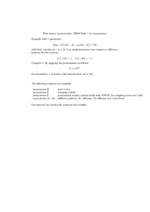
For more information about computing the system matrices, the choice of the output, applying the permutation, please look into the [[media:Readme2.pdf|readme file]]. [[File: Readme2.pdf|thumb]] | For more information about computing the system matrices, the choice of the output, applying the permutation, please look into the [[media:Readme2.pdf|readme file]]. [[File: Readme2.pdf|thumb]] | ||
Example with one parameter: | |||
* <tt>.B</tt>: load vector | |||
* <tt>.E</tt>: heat capacitance matrix | |||
* <tt>.P</tt>: permutation matrix | |||
* <tt>.A</tt>: stiffness matrices (2) | |||
Example with | Example with three parameters: | ||
*.B: load vector | * <tt>.B</tt>: load vector | ||
*.E: | * <tt>.E</tt>: heat capacitance matrices (2) | ||
* <tt>.A</tt>: stiffness matrices (5) | |||
*.A: stiffness matrices ( | |||
To test the quality of the reduced order systems, harmonic simulations as well as transient step responses could be computed, see <ref name="baur11" group="c)"/>. | |||
The output matrix <math>C \in \mathbb{R}^{1 \times 29008}</math> is a vector with non-zero elements <math>C_{173} = 1</math> and <math>C_{133} = -1</math>. | |||
==Dimensions== | |||
System structure (1 parameter): | |||
:<math> | |||
\begin{align} | |||
E \dot{x}(t) &= (A_1 + p (A_2 - A_1)) x(t) + B u(t) \\ | |||
y(t) &= Cx(t) | |||
\end{align} | |||
</math> | |||
System dimensions: | |||
<math>E \in \mathbb{R}^{29008 \times 29008}</math>, | |||
<math>A_{1,2} \in \mathbb{R}^{29008 \times 29008}</math>, | |||
<math>B \in \mathbb{R}^{29008 \times 1}</math>, | |||
<math>C \in \mathbb{R}^{1 \times 29008}</math>. | |||
System structure (3 parameter): | |||
:<math> | |||
\begin{align} | |||
(E_1 + p_0 (E_2 - E_1)) \dot{x}(t) &= (A_1 + p_1 (A_3 - A_1 + A_4 - A_5) + p_2 (A_2 - A_1)) x(t) + B u(t) \\ | |||
y(t) &= Cx(t) | |||
\end{align} | |||
</math> | |||
System dimensions: | |||
<math>E_{1,2} \in \mathbb{R}^{29008 \times 29008}</math>, | |||
<math>A_{1,2,3,4,5} \in \mathbb{R}^{29008 \times 29008}</math>, | |||
<math>B \in \mathbb{R}^{29008 \times 1}</math>, | |||
<math>C \in \mathbb{R}^{1 \times 29008}</math>. | |||
==Citation== | |||
To cite this benchmark, use the following references: | |||
* For the benchmark itself and its data: | |||
::The MORwiki Community, '''Anemometer'''. MORwiki - Model Order Reduction Wiki, 2018. http://modelreduction.org/index.php/Anemometer | |||
@MISC{morwiki_anemom, | |||
author = <nowiki>{{The MORwiki Community}}</nowiki>, | |||
title = {Anemometer}, | |||
howpublished = {{MORwiki} -- Model Order Reduction Wiki}, | |||
url = <nowiki>{https://modelreduction.org/morwiki/index.php/Anemometer}</nowiki>, | |||
year = {2018} | |||
} | |||
* For the background on the benchmark: | |||
==References== | ==References== | ||
a) About the | a) About the '''Anemometer''' | ||
<references group="a)"> | |||
<ref name="ernst01" group="a)">H. Ernst, "<span class="plainlinks">[http://www.freidok.uni-freiburg.de/volltexte/201/ High-Resolution Thermal Measurements in Fluids]</span>," PhD thesis, University of Freiburg, Germany (2001).</ref> | |||
<ref name="benner05" group="a)">P. Benner, V. Mehrmann and D. Sorensen, "<span class="plainlinks">[http://dx.doi.org/10.1007/3-540-27909-1 Dimension Reduction of Large-Scale Systems]</span>", Lecture Notes in Computational Science and Engineering, Springer-Verlag, Berlin/Heidelberg, Germany, 45, 2005.</ref> | |||
<ref name="moosmann05" group="a)">C. Moosmann and A. Greiner, "<span class="plainlinks">[http://dx.doi.org/10.1007/3-540-27909-1_16 Convective Thermal Flow Problems]</span>", Chapter 16 (pages 341--343) of 2.</ref> | |||
</references> | |||
b) MOR for non-parametrized '''Anemometer''' | |||
<references group="b)"> | |||
<ref name="moosmann04" group="b)">C. Moosmann, E. B. Rudnyi, A. Greiner and J. G. Korvink, "<span class="plainlinks">[http://modelreduction.com/doc/papers/moosmann04THERMINIC.pdf Model Order Reduction for Linear Convective Thermal Flow]</span>", | |||
Proceedings of 10th International Workshops on THERMal INvestigations of ICs and Systems, THERMINIC2004, 29 Sept - 1 Oct, 2004, Sophia Antipolis, France.</ref> | |||
</references> | |||
c) MOR for parametrized '''Anemometer''' | |||
<references group="c)"> | |||
<ref name="baur11" group="c)">U. Baur, P. Benner, A. Greiner, J. G. Korvink, J. Lienemann and C. Moosmann, "<span class="plainlinks">[http://dx.doi.org/10.1080/13873954.2011.547658 Parameter preserving model order reduction for MEMS applications]</span>", MCMDS Mathematical and Computer Modeling of Dynamical Systems, 17(4):297--317, 2011.</ref> | |||
<ref name="moosmann07" group="c)">C. Moosmann, "<span class="plainlinks">[http://www.freidok.uni-freiburg.de/volltexte/3971/ ParaMOR - Model Order Reduction for parameterized MEMS applications]</span>", PhD thesis, University of Freiburg, Germany (2007).</ref> | |||
Model Reduction for MEMS | |||
<ref name="moosmann05b" group="c)">C. Moosmann, E. B. Rudnyi, A. Greiner, J. G. Korvink and M. Hornung, "<span class="plainlinks>[http://modelreduction.com/doc/papers/moosmann05MSM.pdf Parameter Preserving Model Order Reduction of a Flow Meter]</span>", Technical Proceedings of the 2005 Nanotechnology | |||
Conference and Trade Show, Nanotech 2005, May 8-12, 2005, Anaheim, California, USA, NSTINanotech | |||
2005, vol. 3, p. 684-687.</ref> | |||
<ref name="rudnyi06" group="c)">E. B. Rudnyi, C. Moosmann, A. Greiner, T. Bechtold, J. G. Korvink, "<span class="plainlinks">[http://modelreduction.com/doc/papers/rudnyi06mathmod.pdf Parameter Preserving Model Reduction for MEMS System-level Simulation and Design]</span>", Proceedings of MATHMOD 2006, February 8 - | |||
10, 2006, Vienna University of Technology, Austria.</ref> | |||
</references> | |||
==Contact== | ==Contact== | ||
[[User: | [[User:Himpe]] | ||
Latest revision as of 08:42, 11 June 2025
| Background | |
|---|---|
| Benchmark ID |
|
| Category |
misc |
| System-Class |
AP-LTI-FOS |
| Parameters | |
| nstates |
29008
|
| ninputs |
1 |
| noutputs |
1 |
| nparameters |
|
| components |
A, B, C, E |
| Copyright | |
| License |
NA |
| Creator | |
| Editor | |
| Location | |
|
NA | |
Description
An Anemometer[a) 1][a) 2][a) 3][c) 1][c) 2][c) 3] (see thermal mass flow meter) is a flow sensing device, consisting of a heater and temperature sensors before and after the heater, placed either directly in the flow or in its vicinity Fig. 1. They are located on a membrane to minimize heat dissipation through the structure. Without any flow, the heat dissipates symmetrically into the fluid. This symmetry is disturbed if a flow is applied to the fluid, which leads to a convection on the temperature field and therefore to a difference between the temperature sensors (see Fig. 2) from which the fluid velocity can be determined.
The physical model can be expressed by the convection-diffusion partial differential equation [b) 1]:
where denotes the mass density, is the specific heat capacity, is the thermal conductivity, is the fluid velocity, is the temperature, and is the heat flow into the system caused by the heater.
The solid model has been generated and meshed in ANSYS. Triangular PLANE55 elements have been used for the finite element discretization. The order of the system is .
Example with one parameter:
The dimensional ODE system has the following transfer function
with the fluid velocity as single parameter. Here is the heat capacitance matrix, is the load vector which is derived from separating the spatial and temporal variables in and the FEM discretization w.r.t. the spatial variables. are the stiffness matrices with for pure diffusion and for diffusion and convection. Thus, for obtaining pure convection you have to compute .
Example with three parameters:
Here, all fluid properties are identified as parameters. Thus, we consider the following transfer function
with parameters , , which are combinations of the original fluid parameters , , , : , , and , see [c) 4]. So far, we have considered the mass density as fixed, i.e. .
Origin
- IMTEK Freiburg, Simulation group, Prof Dr Jan G. Korvink has taken on a position as Director of the Institute of Microstructure Technology (IMT) at the Karlsruhe Institute of Technology (KIT).
Data
Matrices are in the Matrix Market format. All matrices (for the one parameter system and for the three parameter case) can be found and uploaded in Anemometer.tar.gz. The matrix name is used as an extension of the matrix file. The system matrices have been extracted from ANSYS models by means of mor4fem.
For more information about computing the system matrices, the choice of the output, applying the permutation, please look into the readme file.
Example with one parameter:
- .B: load vector
- .E: heat capacitance matrix
- .P: permutation matrix
- .A: stiffness matrices (2)
Example with three parameters:
- .B: load vector
- .E: heat capacitance matrices (2)
- .A: stiffness matrices (5)
To test the quality of the reduced order systems, harmonic simulations as well as transient step responses could be computed, see [c) 4].
The output matrix is a vector with non-zero elements and .
Dimensions
System structure (1 parameter):
System dimensions:
, , , .
System structure (3 parameter):
System dimensions:
, , , .
Citation
To cite this benchmark, use the following references:
- For the benchmark itself and its data:
- The MORwiki Community, Anemometer. MORwiki - Model Order Reduction Wiki, 2018. http://modelreduction.org/index.php/Anemometer
@MISC{morwiki_anemom,
  author =       {{The MORwiki Community}},
  title =        {Anemometer},
  howpublished = {{MORwiki} -- Model Order Reduction Wiki},
  url =          {https://modelreduction.org/morwiki/index.php/Anemometer},
  year =         {2018}
}
- For the background on the benchmark:
References
a) About the Anemometer
- ↑ H. Ernst, "High-Resolution Thermal Measurements in Fluids," PhD thesis, University of Freiburg, Germany (2001).
- ↑ P. Benner, V. Mehrmann and D. Sorensen, "Dimension Reduction of Large-Scale Systems", Lecture Notes in Computational Science and Engineering, Springer-Verlag, Berlin/Heidelberg, Germany, 45, 2005.
- ↑ C. Moosmann and A. Greiner, "Convective Thermal Flow Problems", Chapter 16 (pages 341--343) of 2.
b) MOR for non-parametrized Anemometer
- ↑ C. Moosmann, E. B. Rudnyi, A. Greiner and J. G. Korvink, "Model Order Reduction for Linear Convective Thermal Flow", Proceedings of 10th International Workshops on THERMal INvestigations of ICs and Systems, THERMINIC2004, 29 Sept - 1 Oct, 2004, Sophia Antipolis, France.
c) MOR for parametrized Anemometer
- ↑ C. Moosmann, "ParaMOR - Model Order Reduction for parameterized MEMS applications", PhD thesis, University of Freiburg, Germany (2007).
- ↑ C. Moosmann, E. B. Rudnyi, A. Greiner, J. G. Korvink and M. Hornung, "Parameter Preserving Model Order Reduction of a Flow Meter", Technical Proceedings of the 2005 Nanotechnology Conference and Trade Show, Nanotech 2005, May 8-12, 2005, Anaheim, California, USA, NSTINanotech 2005, vol. 3, p. 684-687.
- ↑ E. B. Rudnyi, C. Moosmann, A. Greiner, T. Bechtold, J. G. Korvink, "Parameter Preserving Model Reduction for MEMS System-level Simulation and Design", Proceedings of MATHMOD 2006, February 8 - 10, 2006, Vienna University of Technology, Austria.
- ↑ 4.0 4.1 U. Baur, P. Benner, A. Greiner, J. G. Korvink, J. Lienemann and C. Moosmann, "Parameter preserving model order reduction for MEMS applications", MCMDS Mathematical and Computer Modeling of Dynamical Systems, 17(4):297--317, 2011.